What is Polar Coordinates?
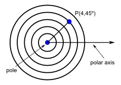
The polar coordinate system is a way to graph a point in two dimensions just like the Cartesian system. This system is based on a central point called the pole (the origin in the Cartesian system) and an axis extending in a positive direction from the pole called the polar axis (the x-axis in the Cartesian system). A point is defined by the ordered pair (r, theta) where r is the distance from the pole and theta is the angle between the polar axis and the line made between the point and the pole.
Here's an example:
While traditional algebraic functions can be graphed on a polar coordinate system, trigonometric functions reveal particularly interesting results.
Polar coordinates are used extensively in nagivation. They are also used for modeling systems that display radial symmetry like ground water flow, or radial force like gravitational fields.
How Do I Use This Activity?
This activity allows the user to plot ordered pairs and algebraic or trigonometric functions on the same polar coordinate plane.
Controls and Output
-
The area at the top of the screen is where the plot is displayed.
-
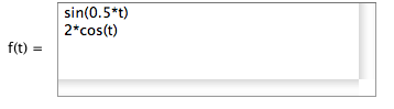
The Function area is for entering functions. To graph a function, type the formula of the function you want to graph in the space at the bottom of the applet, next to "f(t) =" where t represents theta. You may graph up to 10 functions on the same plot. To graph multiple functions enter one formula per line, as shown.
Basic functions and their compositions can be typed as follows:
Function Symbol Examples Meaning addition + x + 3 x plus three subtraction - 5 - x five minus x multiplication * x*(x - 2) x times the quantity x minus two division / 3/x three divided by x power ^ x^3 x to the power of three (pi) pi sin(pi*x) sin of the quantity (pi) times x square root sqrt(...) sqrt(x) square root of x nth root* x^(1/n) x^(1/3) cube root of x absolute value abs(...) abs(3 - x) absolute value of the quantity three minus x e to the power of x exp(...) exp(x) e to the power of x sine sin(...) sin(x) sine of x cosine cos(...) cos(5 - x) cosine of the quantity five minus x tangent tan(...) tan(x) tangent x arcsine asin(...) 2*asin(x) two times arcsine x arccosine acos(...) acos(x) arccosine x arctangent atan(...) atan(x) arctangent of x hyperbolic sine sinh(...) sinh(x) hyperbolic sine of x hyperbolic cosine cosh(...) cosh(10/x) hyperbolic cosine of the quantity ten divided by x hyperbolic tangent tanh(...) tanh(x) hyperbolic tangent of x natural logarithm ln(...) ln(x) natural logarithm of x base 10 logarithm log(...) log(x + 5) base ten logarithm of the quantity x plus five NOTE: For functions where there is a range of values for which the function is undefined, this application will draw a straight line over the range which is undefined.
-
The
Data area is for entering data points. Data points should be in the form (r, theta). A space or
a carriage return is required to separate the data points from one another. After you input
the coordinates, you must press the
Plot/Update button to graph them.

If you have trouble copying data from the applet and pasting it into an Excel spreadsheet, please see our Excel Copy/Paste Help.
If the Use Radians option is chosen, values for theta can be input using the word pi, as in pi/4 or 2pi/3. You can also use the functions listed in the table above to create values for r.
If the values for r or theta are negative, they will be converted to appropriate positive values. If the value of theta is greater than 2 pi, then it will be converted to the appropriate value less than or equal to 2 pi.
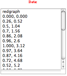
- Just as you can plot up to 10 functions at once, you can also plot up to 12 data sets at the same time. Separate multiple data sets by typing newgraph on a line by itself in the Data window. If you want to specify your own colors for the graphs you can replace newgraph with the following keywords: bluegraph, redgraph, greengraph, graygraph, magentagraph, orangegraph, purplegraph, crimsongraph, blackgraph, browngraph, darkbluegraph.
-
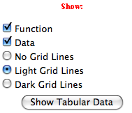
You can choose what you see on the graph. You can select to show all functions, all data, and/or the grid lines by checking the appropriate box or radio button in the Show box.
-
The applet also can tell you the location of any click. Just click the mouse anywhere on the
graph and the coordinates will appear in the
Mouse Position box.

-
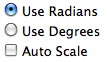
Auto Scale: Checking the Auto Scale check box gives the smallest window possible so that all of the
data points still fit on the coordinate plane. (
NOTE: There must be data for this feature to work. ) You can also choose whether data is given in
radians or degrees. If you choose degrees, the value of t will be given in degrees when you
choose to show tabular data.
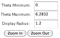
- Theta Minimum and Theta Maximum allow the user to adjust the range of the function.
-
The Display Radius allows the user to manually adjust the size of the viewing window. The user may also use the Zoom In and Zoom Out buttons to control this. Since polar coordinates are defined by distance from the pole and angle from the polar axis, the viewing window always remains square with the pole at the center.
-
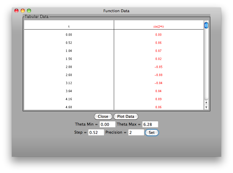
To view a table of values corresponding to the graphed function, click the Show Tabular Data button.

-
The t values in the table increment equally and then give the corresponding f(t) values for
each function plotted. You can change these data values by entering a new theta minimum
value, new theta maximum value, and step size, all of which should be expressed in radians.
If you enter a step that does not divide evenly into the range, the table will stop at the
greatest multiple of the step that is less than the maximum. The precision field allows you
to adjust the number of decimal points displayed.
-
When the Plot Data button within the Show Tabular Data window is pressed, the data listed in tabular form in the Tabular Data window is plotted on the graph of the main screen.
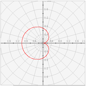
Graph of sin(.5*t) in red and sin(2t) in blue:
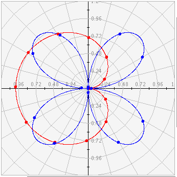
In addition to plotting the data on the graph, the text area is populated with text corresponding to the data points plotted.
Description
This activity allows the user to plot ordered pairs and algebraic or trigonometric functions on the polar coordinate plane. This activity would work well in groups of two to four for about forty-five minutes if you use the exploration questions and twenty minutes otherwise.
Place in Mathematics Curriculum
This activity can be used to:
- introduce the polar coordinate system
- practice students' point plotting skills
- demonstrate conversion between radians and degrees
Standards Addressed
Grade 9
-
Functions and Relationships
- The student demonstrates conceptual understanding of functions, patterns, or sequences including those represented in real-world situations.
- The student demonstrates algebraic thinking.
Grade 10
-
Functions and Relationships
- The student demonstrates conceptual understanding of functions, patterns, or sequences including those represented in real-world situations.
- The student demonstrates algebraic thinking.
Grades 8-12
-
Mathematical Analysis
- 1.0 Students are familiar with, and can apply, polar coordinates and vectors in the plane. In particular, they can translate between polar and rectangular coordinates and can interpret polar coordinates and vectors graphically.
-
Trigonometry
- 15.0 Students are familiar with polar coordinates. In particular, they can determine polar coordinates of a point given in rectangular coordinates and vice versa.
- 16.0 Students represent equations given in rectangular coordinates in terms of polar coordinates.
- 17.0 Students are familiar with complex numbers. They can represent a complex number in polar form and know how to multiply complex numbers in their polar form.
Secondary
-
AP Calculus
- APC.08 The student will apply the derivative to solve problems. This will include analysis of curves and the ideas of concavity and monotonicity; optimization involving global and local extrema; modeling of rates of change and related rates; use of implicit differentiation to find the derivative of an inverse function; interpretation of the derivative as a rate of change in applied contexts, including velocity, speed, and acceleration; and, differentiation of nonlogarithmic functions, using the technique of logarithmic differentiation. * * AP Calculus BC will also apply the derivative to solve problems. This will include analysis of planar curves given in parametric form, polar form, and vector form, including velocity and acceleration vectors; numerical solution of differential equations, using Euler's method; l'Hopital's Rule to test the convergence of improper integrals and series; and, geometric interpretation of differential equations via slope fields and the relationship between slope fields and the solution curves for the differential equations.
- APC.09 The student will apply formulas to find derivatives. This will include derivatives of algebraic, trigonometric, exponential, logarithmic, and inverse trigonometric functions; derivations of sums, products, quotients, inverses, and composites (chain rule) of elementary functions; derivatives of implicitly defined functions; and, higher order derivatives of algebraic, trigonometric, exponential, and logarithmic, functions. * * AP Calculus BC will also include finding derivatives of parametric, polar, and vector functions.
- APC.15 The student will use integration techniques and appropriate integrals to model physical, biological, and economic situations. The emphasis will be on using the integral of a rate of change to give accumulated change or on using the method of setting up an approximating Riemann sum and representing its limit as a definite integral. Specific applications will include the area of a region; the volume of a solid with known cross-section; the average value of a function; and, the distance traveled by a particle along a line. * * AP Calculus BC will include finding the area of a region (including a region bounded by polar curves) and finding the length of a curve (including a curve given in parametric form).
-
Mathematical Analysis
- MA.10 The student will investigate and identify the characteristics of the graphs of polar equations, using graphing utilities. This will include classification of polar equations, the effects of changes in the parameters in polar equations, conversion of complex numbers from rectangular form to polar form and vice versa, and the intersection of the graphs of polar equations.
Be Prepared to
- explain the difference between cartesian coordinates and polar coordinates
- explain the difference between radians and degrees
- explain periodic functions