Parametric GraphIt

What is Parametric GraphIt?

This activity allows the user to plot ordered pairs and parametric equations on the same coordinate plane. The applet is similar to GraphIt except you have to input the parametric representation of a function instead of the regular function.

Parametric equations are a way to represent functions and other graphs by using separate equations for each coordinate. This is done to give a direction, or orientation, to a theoretical object traveling along the curve. Instead of there being a function where y depends on x, there are two equations x(t) and y(t) which both depend on t. The variable t is called the parameter and the two equations for x and y are called the parametric equations. The points on the graph have coordinates (x(t), y(t)) for some range of t.

Parametric equations have the ability to present graphs that wouldn't pass the vertical line test for functions. Functions can easily be represented by parametric equations but not all sets of parametric equations can be represented by functions. The following is the graph of y=.5x^3 represented by the parametric equations x(t)=t and y(t)=.5t^3.

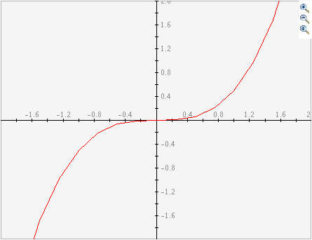
To represent a function with its parametric equations, simply set x(t)=t and y(t)= the original function.

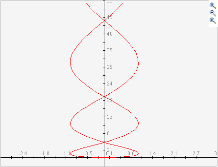
The following is a graph of the parametric equations x(t)=sin(t) and y(t)=.5t^2. This cannot be represented as a function because it fails the vertical line test.

Related Resources

• Activity Graphit
• Activity Vertical Line Test
• Discussion about Functions and the Vertical Line Test
• Worksheet Parametric GraphIt Exploration Questions
• Worksheet Parametric GraphIt Exploration Questions (doc)

How Do I Use This Activity?

This activity allows the user to plot ordered pairs and parametric equations on the same coordinate plane.

Controls and Output

• The area at the top of the screen is where the plot is displayed.

• The Equation area is for entering equations for x and y. To graph parametric equations, type the equation for x and y in the text boxes next to x= and y= respectively. Make sure the equations are a function of t since parametric equations are graphed with respect to time. You may graph up to four equations on the same plot. Enter one formula per line, as shown.

• Basic functions and their compositions can be typed as follows:
  
  

  Function	Symbol	Examples (including combinations of functions)
  addition	+	t + 3 t plus three
  subtraction	-	5 - t five minus t
  multiplication	*	(t - 2)*t t times t minus two
  division	/	3/t three divided by t
  power	^	t^3 - 1 t to the power of three minus one
  power	**	t**3 - 1 t to the power of three minus one
  (pi)	pi	sin(pi*t) sin of (pi) times t
  square root	sqrt(...)	sqrt(t-1) square root of t minus one
  nth root (see * below)	t^(1/n)	t^(1/3) cube root of t
  absolute value	abs(...)	abs(3 - t) absolute value of three minus t
  e to the power of t	exp(...)	exp(t) e to the power of t
  sine	sin(...)	sin(t**2) sine of t squared
  cosine	cos(...)	cos(5 - t) cosine of five minus t
  tangent	tan(...)	tan(t) tangent t
  arcsine	asin(...)	2*asin(t) two times arcsine t
  arccosine	acos(...)	acos(t) arccosine t
  arctangent	atan(...)	atan(t) arctangent of t
  hyperbolic sine	sinh(...)	sinh(1 - t) hyperbolic sine of one minus t
  hyperbolic cosine	cosh(...)	cosh(10/t) hyperbolic cosine of ten divided by t
  hyperbolic tangent	tanh(...)	tanh(t) hyperbolic tangent of t
  natural logarithm	ln(...)	ln(t) natural logarithm of t
  base 10 logarithm	log(...)	log(t + 5) base ten logarithm of t plus five

  
  
  
• The Data area is for entering data points. Data points should be in the form (x,y). Parentheses around the data point are optional. A tab or a space can separate the x and the y though no space is needed. A space or a carriage return is required to separate the data points from one another. After you input the coordinates, you must press the Plot/Update button to graph them.
  
  
• If you have trouble copying data from the applet and pasting it into an Excel spreadsheet, please see our Excel Copy/Paste Help.
  
  
• You can plot a total of four pairs of equations at once. You can also plot a total of twelve data sets at once. Separate each function with a comma or by starting a new line. Separate data sets by typing newgraph on a line by itself in the Data window. If you want to specify your own colors for the graphs you can replace newgraph with the following keywords: bluegraph, redgraph, greengraph, blackgraph, graygraph, magentagraph, browngraph, orangegraph, purplegraph, crimsongraph, darkbluegraph.
  
  
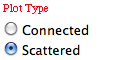
• You can choose from two plot types. Connected draws a line from one point to the next. Scattered just draws the points as dots on the graph. These options do not affect the way equations are graphed.
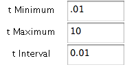
• Since parametric equations are functions of time, you can adjust the starting and ending time as well as the interval. To do this, adjust the values in t Minimum, t Maximum, and t Interval.
• Click Set Window to determine how the coordinate plane will appear on your screen. A new window will open that allows you to change the settings. X min and X max are the minimum and maximum x-values displayed on the graph. Similarly, Y min and Y max are the minimum and maximum y-values. X scale and Y scale are the distances between vertical and horizontal gridlines. If you choose Choose Scale Automatically, a reasonable scale will be chosen for you, otherwise you can uncheck the box and select your own scale. If at anytime you want to restore the default window, click on the Get Defaults button. Click Set to make the changes to the window parameters take effect.
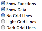
• You can choose what you see on the graph. You can select to show all functions, all data, and/or the grid lines by checking the appropriate box or radio button in the Show box.
• The applet can also tell you the location of any click. Just click the mouse anywhere on the graph that you want to know the coordinates of and the coordinates will appear in the Mouse Position box.
• Zoom/Pan buttons: In the upper right corner of the graph, there are three buttons with pictures of magnifyng glasses. From top to bottom these buttons represent zoom in, zoom out, and pan, respectively.
  
  
  • To zoom in, click the top button to depress, then click and drag over the area of the graph for which you wish to zoom to. Note that after clicking and dragging over the selected area, the zoom in button is automatically released.
  • To zoom out, simply click the middle button. The graph will automatically zoom out by doubling the min and max values of the axes.
    
    
  • To use the pan feature, click the bottom magnifying glass button to depress it. Click and drag over the graph and the graph will pan around according to the movement of the mouse. Upon releasing the mouse, the pan button is released.
    
    
  • Checking the Auto Scale check box gives the smallest window possible so that all of the data points still fit on the coordinate plane. Note that there must be data for this feature to work.
    
    
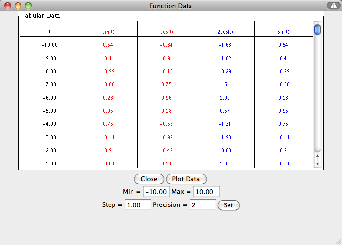
• To view a table of values corresponding to the graphed function, click the Show Tabular Data button.
• The t values in the table increment equally and then give the corresponding x(t) and y(t) values for each equation plotted. You can change these data values by entering a new minimum t value, new maximum t value, and step size. If you enter a step that does not divide evenly into the range, the table will stop at the greatest multiple of the step that is less than the maximum. The precision field allows you to adjust the number of decimal points displayed.
  
  
• When the Plot Data button within the Show Tabular Data window is pressed, the data listed in the Tabular Data window is plotted on the graph of the main screen.