Recursion

What is Recursion?

This activity allows the user to graph up to three recursive equations at one time.

In a recursive equation, each value u _n depends on the value before it u _n-1 . The n is just a counting number to keep track of which value comes after which. So the initial value is said to be u ₀ where n=0. The next value is u ₁ , the next u ₂ and so on. Once the initial value is established, some computation is performed to it producing the value for u ₁ . The same computation is then performed to u ₁ to produce u ₂ , which then produces u ₃ and so on.

For example let's look at the recursive equation u _n = u _n-1 + 2 with the initial value u ₀ =0. To find u ₁ we use the equation and take n to equal 1. So u ₁ = u _1-1 + 2 = u ₀ + 2 = 0 + 2 = 2. Therefore u ₁ = 2. To find u ₂ we use the value of u ₁ to find u ₂ = u ₁ + 2 = 2 + 2 = 4.

In this activity the user must write a recursive equation involving u _n equal to some computation to u _n-1 (ie u _n = u _n-1 + 2). The initial values u ₀ must also be specified. adjusted by the user to understand their role in the graph of the equation. This activity uses the first 10 iterations of the equations to make up the points of the graph. On the graph the points are connected enabling the user to view the overall trend of each graph. The user may then flip through each equation on the graph and view the value at each graphed point.

When we normally think of an equation, we think of something like y = 2*x, where you plug in any value for x and receive a unique y value. Notice to receive a value, no previous value needs to be calculated. This is not the case in a recursive equation. A recursive relationship simply means that each value of the function is determined by the previous value.

In recursive equations, each value is determined by the previous value. An initial number is needed in order for first value to be found. So the initial value is placed into the equation to get the first value. Then that first value is inputted into the equation to get the second value and so on. This process will occur up until the number of iterations that the user has specified.

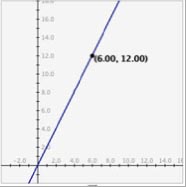
For example, let's use the recursive equation u _n = u _n-1 + 2. We must also specify the initial value, which we will set as u ₀ = 0. Let's compare these results to that of the function f(x) = 2*x:

u n = u n-1 + 2	f(x) = 2 * x
u 0 = 0 u 1 = 2 u 2 = 4 u 3 = 6 u 4 = 8 u 5 = 10 u 6 = 12 u 7 = 14 u 8 = 16 u 9 = 18

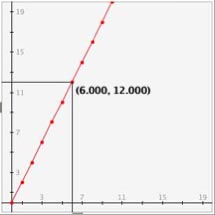
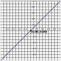
Notice that this graph is similar to that of that of the function f(x) = 2*x. If you start plugging in the integer values 0-5 into the function f(x) = 2*x, you receive the exact values of the recursive equation u _n = u _n-1 + 2. Why is this the case? Let's look at the values for the 3rd position on the graph. For the function: f(3) = 2*3 = 6. Remember the recursive equation u _n = u _n-1 + 2. Then u ₃ = u ₂ + 2. But what is the value for u ₂ ? Well u ₂ = u ₁ + 2. So u ₃ = (u ₁ + 2) + 2. And u ₁ = u ₀ + 2. Then u ₃ = ((u ₀ + 2) + 2) + 2. Since we know that u ₀ = 0, we can calculate the value. u ₃ = ((0 + 2) + 2) + 2 = 6. We are adding 2 three times. This is the same as 2*3 which was the value for the function.for an x number of times. So there is a direct relationship between the linear function and the recursive function.

Recursive equations are important to understand because they occur in many everyday situations. Many of these occurrences involve recursive equations more complicated than the one that we just investigated. The non-recursive function is not always so easy to derive. A common recursive equation is one involving compounding interest. Let's use an example. Sally initially puts $1000 into a savings account that gives her .07% interest every year. This means each new year she would receive an additional .07% of what she had the previous year. This situation can be represented in the formula: u _n = u _n-1 * (1 + .0007). Where u ₀ = 1000. The number of iterations would be the number of years she had her money in this savings account.

This graphing activity may be used for real world examples such as compounding interest. Also the activity can be used for all kinds of recursive equations. Since the activity creates a graph, the user becomes able to compare the equations to more familiar equations. Furthermore, the user is able to connect the abstract ideas of recursion to a concrete visual graph.

Related Resources

• Activity Hilbert Curve Generator
• Activity Koch's Snowflake
• Activity Sequencer
• Activity Sierpinski's Carpet
• Activity Sierpinski's Triangle
• Discussion about Properties of Fractals
• Discussion about Recursion
• Worksheet Recursion Exploration Questions
• Worksheet Recursion Exploration Questions (doc)

How Do I Use This Activity?

This activity allows the user to graph recursive equations. The user specifies both the initial value and the recursive function for up to three equations. This activity uses the first 10 iterations of the equations to draw as points on the graph. The user may then flip through each equation on the graph and view the value at each graphed point.

Controls and Output

For the Equations Page:

• The user may enter up to three equations on this page. The equations are referred to as "Relations."
• Each equation has its own variable. There is a default letter and initial value for each variable. If the user wishes to change the letter, he or she may enter a letter into the text box just following the Set Variable button. The user may also change the initial value of the variable by typing in a number next to the u ₀ =. Then the user should click the Set Variable button to change the letter throughout the relation.
  

  Notice that to make a valid recursive equation, the same letter must be used in the equation. So if the variable is the letter a, the equation should remain consistent like in the following example:

  • The user must enter in an equation. This is done in the text box next to the symbols u _n = _n ) depend on the last value of the variable (u _n-1 ).

    
• To achieve subscripted text, the user simply types the dependant variable then n-1. The activity is programmed to subscript the n-1. Once the relation includes a string in the form u _n-1 (or another dependent varaible determined by the user) it becomes a valid recursive equation.
• When the Clear Equation button is clicked, both the equation typed into the text box and the equation appearing in the text field are cleared.
  
• Once the user is satisfied with the variables and equations for each relation, he or she may click the Graph it! button at the top of the page to see the graphs of the equations.

For the Graphs Page:

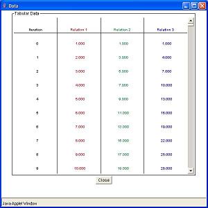
• To view all the data points at once click the Show Data button. Then a chart appears in a separate window listing each data point in a chart.

  
  

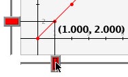
• To navigate the graph use the slider bars on the bottom and left side of the graph. Click on the central rectangle and drag across. For the slider bar on the bottom drag left and right, for the one on the left side drag up and down. Notice that both slider bars move and they attach to the point closest to the slider bar. The value that appears on the screen is that of the point to which the slider bar is currently attached.

  

• The user can switch between equations so that they can view their values one at a time. They can do this by using the drop down menu located below the graph.

  

• The user can also change how they want the graph displayed. If you check the Connect data points check box the points will be connected by a line. The default connects the points so that you can better view the shape of the graph. If you check the Fit graph size to data points check box the graph will resize to fit all the data points.
  
• There are three types of grids: No Grid, Light Grid Lines, and Dark Grid Lines. To activate any of these three options, highlight the circle next to the appropriate option:
  

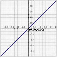
  No Grid graph:	Light Grid Line graph:	Dark Grid Grid Line graph: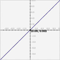

• There are two ways to alter the range on the axes.
  1. Setting exact values for axis mins/maxes: You may set the graph boundaries by clicking the Preferences button and entering new values for the x max, x min, y max, y min, or iterations. Then click the Set Window button to set the boundaries. To return the values to their defaults, you click the Get Defaults button and then click the Set button again. If you do not want to change the window settings you may click Cancel.
     
  2. Zoom/Pan buttons: In the upper right corner of the graph, there are three buttons with pictures of magnifying glasses. From top to bottom these buttons represent zoom in, zoom out, and pan, respectively.
     • To zoom in, click the top button to depress it, then click and drag over the area of the graph that you wish to magnify. The images below show first the process of dragging a box around a desired zoom area with the mouse (left), and then the resulting zoomed image after the mouse button is released (right). Note that after the zoom-in has been performed, the zoom-in button at top right is no longer depressed.
       _
     • To zoom out, simply click the second of the three zoom buttons. The graph will automatically zoom out by doubling the min and max values of the axes.
     • To use the pan feature, click the bottom magnifying glass button to depress it. Click and drag over the graph and the graph will pan around according to the movement of the mouse. Upon releasing the mouse, the pan button is released.
• The user can also go back and change the recursive equations at any time by clicking on the Back button.
  

Description

This activity allows the user to explore different recursive equations. This activity would work well in small groups of 2-3 for about 40 minutes if you use the exploration questions and 20 minutes otherwise.

Place in Mathematics Curriculum

This activity can be used to:

• Teach students about recursive equations
• Show up to three recursive equations on a graph
• Trace individual values of a recursive equation using a graph

Be Prepared to

• provide a variety of recursive equations for students to try, for example experiment withmultiplying and dividing.
• encourage students to test different initial values
• connect recursive equations to real life examples such as compounding interest
• show students how to read the graph and trace the values of the recursive equation at each pointand switch from one equation to the next

Related Resources

• Activity Hilbert Curve Generator
• Activity Koch's Snowflake
• Activity Sequencer
• Activity Sierpinski's Carpet
• Activity Sierpinski's Triangle
• Discussion about Properties of Fractals
• Discussion about Recursion
• Lesson on An Introduction to Arithmetic and Geometric Sequences
• Lesson on Introduction to Fractals: Infinity, Self-Similarity and Recursion
• Lesson on Properties of Fractals
• Worksheet Recursion Exploration Questions
• Worksheet Recursion Exploration Questions (doc)