Spread of Disease

What is Spread of Disease?

This activity allows the user to model a population of people susceptible to a disease, infected with the disease, and recovered from the disease. It demonstrates what happens in the real world when people infected with a contagious disease interact with others in their community.

When an infected person meets a susceptible person (someone who is able to get that disease), there is a certain chance that the disease will spread to the susceptible person, and he or she will become infected. Infected people are sick for a certain number of days, and after that period, there is a certain chance they will recover. After that, they will be immune to the disease for a certain period of time, but they can become susceptible again later. The rules of the applet are:

• Whenever an infected person is in a square next to a susceptible person, there is a certain probability that the susceptible person will become infected. (Note: the person will not become sick if an infected person is in a square diagonal to them.)
• After a certain number of days, the infected person has a chance, each day, to recover.
• Then, after another number of days, that person has a chance, each day, to become susceptible again.

Using this model, you can see how a population is affected by a contagious disease depending on different characteristics of the disease and population. Try experimenting with different characteristics of the disease like infection rate, initial population, etc. to see what happens to the population with different parameters. Do the results change when the parameters change? Are they always the same with the same parameters? What does this tell you about how real-world populations react to disease?

This model was based on a model created in NetLogo, so if you have NetLogo, you could try making a more simple or more complex version on your own. NetLogo is free to download here. You could try making the model from scratch, or you can download a text file of the code ( Download File). You will still have to create the buttons and slider bars manually. Or, you can download the entire model ( Download File) with slider bars and buttons (but a simpler version). Try adding or subtracting your own parameters to the model to see how it affects the population.

Related Resources

• Activity A Better Fire!!
• Activity Advanced Fire
• Activity Directable Fire!!
• Activity Fire!!
• Activity Rabbits and Wolves
• Discussion about Chaos
• Discussion about Chaos is Everywhere
• Worksheet Spread of Disease Exploration Questions
• Worksheet Spread of Disease Exploration Questions (doc)

How Do I Use This Activity?

This activity allows the user to model a population of people susceptible to a disease, infected with the disease, and recovered from the disease.

Controls and Output

The main grid is where you can see your settings modeled on a population of people who are either susceptible to a disease, infected with the disease or recovered from the disease. The population always begins with one infected person, while the rest are susceptible. The grid shown below shows a day in the progression of the disease when some people are susceptible (orange), some are infected (green), and others are recovered (blue).

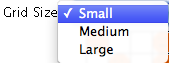
You can adjust the size of the grid by using the Grid Size drop down menu:

You can control how the borders of the grid behave by setting the Grid Border to either Island or Toroid. The Island border behaves like an island in that when a person encounters the border, they cannot continue in the same direction. With a Toroid border, when a person encounters a border and continues to move in the same direction, they appear on the opposite side of the grid as if the two sides were connected. Toroid is similar to viewing Earth on a flat map.

Clicking on the View Population Graph button will display a graph of the number of susceptible, infected, and recovered people over time.
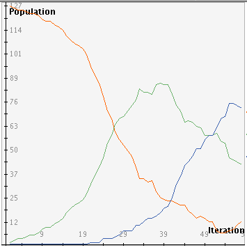
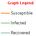
The legend below the graph explains which color represents each type of person.
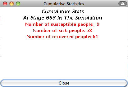
Clicking on View Cumulative Stats brings up a popup box with the number of stages that have progressed and the current number of susceptible, sick, and recovered people.

Clicking on View Simulation Key brings up a popup box with a legend of all the terms and icons needed to understand the SIR Model.

You change the settings of the model by clicking View/Modify Parameters. This will open a dialog box where you can change settings using the input boxes.

• The Sick Rate box determines the probability that, when an infected person is next to a susceptible person, the susceptible person will become infected.
• You can change the population size using the Initial Population box. The range is 2 to 1936, but the maximum depends on the size of the grid. This number can be altered while the simulation is running, but changes will not take effect until the simulation is reset.
• You can adjust the recovery rate using the Recovery Rate box. The recovery rate determines the probability that an infected person will recover after the specified number of "days to recovery".
• You can determine how many days it takes someone to recover from the disease using the Days to Recovery box. After that number of 'days' or timesteps, the person will either recover or remain sick based on the recovery rate probability.
• The susceptibility rate is determined by the Susceptibility Rate box, and it sets the probability that a recovered person will become susceptible again after the number of 'days to susceptibility' that you specify.
• The Days to Susceptibility box controls the number of days someone must be recovered before they can again become susceptible to the disease.

Description

This activity allows the user to model a population of people susceptible to a disease, infected with the disease, and recovered from the disease. It demonstrates what happens in the real world when people infected with a contagious disease interact with others in their community. This activity would work well in groups of two to four for about thirty minutes if you use the exploration questions and ten to fifteen minutes otherwise.

Place in Mathematics Curriculum

This activity can be used to:

• demonstrate randomness
• motivate the idea of chaos
• demonstrate concepts of probability
• motivate data analysis
• provide a data set for use with graphing tools

Be Prepared to

• define susceptibility and explain how it is functioning in this activity
• encourage students to experiment with different parameters
• explain why the results are different even though the same parameters are used
• help students interpret the graph that displays the model's results

Related Resources

• Activity A Better Fire!!
• Activity Advanced Fire
• Activity Directable Fire!!
• Activity Fire!!
• Activity Rabbits and Wolves
• Discussion about Chaos
• Discussion about Chaos is Everywhere
• Lesson on Chaos
• Worksheet Spread of Disease Exploration Questions
• Worksheet Spread of Disease Exploration Questions (doc)