Multi-Function Data Flyer

What is Multi-Function Data Flyer?

This activity allows the user to plot a set of (x,y) ordered pairs and graph a function on the same coordinate plane. The applet allows the manipulation of a function of the form y = f(x). Using slider bars one can manipulate the function to change the constant values and view the effects of those changes.

The user can explore the effect of changing constants in most types of functions including:

• linear
• quadratic
• exponential
• trignometric

If an equation has the addition of a number, such as in the equation y=ax+b, then manipulating the number that is added on (in this case, variable 'b') will always cause the graph to move up and down along the y-axis. By adding a multiplier, variable 'a' in this example, the graph will expand and retract as the variable is manipulated. Experiment with the slider tabs and see if you can find any other patterns.

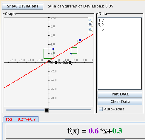
The sum of the squares of the deviations is shown to assist the user in determining how well the function fits the data. As a general rule of thumb, the smaller this value, the better the curve fits the data for that type of function. However, this value implies little about the goodness of fit between different functions.

Related Resources

• Activity Conic Flyer
• Activity Data Flyer
• Activity Derivate
• Activity Function Flyer
• Activity Function Revolution
• Activity Graphit
• Activity InteGreat!
• Activity Multiple Linear Regression
• Activity Overlapping Gaussians
• Discussion about From Graphs to Function Machines and Back
• Discussion about Functions as Processes or Rules: "Function Machines"
• Discussion about Independent and Dependent Variables
• Worksheet Multi-Function Data Flyer Exploration Questions
• Worksheet Multi-Function Data Flyer Exploration Questions (doc)

How Do I Use This Activity?

This activity allows the user to plot coordinate pairs and one or more algebraic functions on the same coordinate plane with the ability to use sliders to manipulate the constants of the graphed functions.

Controls and Output

Find out about...

Entering Functions

• The Multi-Function Data Flyer allows you to enter algebraic functions in the box labeled f(x)=. For information on the syntax of entering functions and numbers with scientific notation, see Interactivate Functions Help.

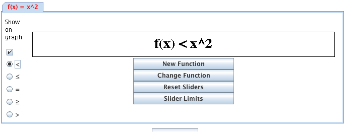
• Enter the function you want to graph in the box marked f(x)=. Enter constants or coefficients as either a number or letter. The computer will recognize anything in the equation that is not the independent variable as a parameter. For instance, if you wish to experiment with the linear function f(x) = x + 8 and wish to manipulate the coefficient of x as well as the constant, it is necessary to type the equation as something like f(x) = 1x + 8 or f(x)=ax+b. If you want to experiment with the sine function f(x) = sin(x) and be able to manipulate the parameters such as the y-intercept, phase, frequency, and amplitude, it is necessary to type something like 1sin(1x+0)+0 or f(x)=asin(bx+c)+d. Click Set Function to graph the function. At this point, radio buttons will appear, allowing you to change the function to an inequality. The function will initially be graphed as an equality, but as you click on the inequality radio buttons, the graph will change to reflect your choice. See the picture below.

  

• If you wish to enter multiple functions, you do not need to retype f(x)=. Simply place a semi-colon between the functions you want to graph. See the picture below.
  
• Note that numerical values entered should be accurately calculated from 10 ^-8 to 10 ⁸ . Numbers larger or smaller than these values produce unreliable results. If you enter a number with a magnitude smaller than 10^-6 or larger than 10^6 it will automatically be converted to scientific notation.
• This activity also allows you to choose from pre-defined functions so you do not need to type in the function. Click on the Preset Functions button and then select the function you wish to graph from the window that opens. Click on the image of the function and then click the Set button. This inserts the equation of the function into the text box. Close the window by clicking the Close button and then click the Set Function button to graph it.
• There are several additional checkboxes on this screen that control various aspects of the function. These checkboxes, located to the right of where the function is input, include: Exponents Change, Use Multi-Letter Variables, and Unlink Variables.
  • The Exponents Change checkbox, when checked, will create a slider bar for any exponent in the function. If left unchecked, a slider will not be available for the exponents when the function is graphed.
  • The Use Multi-letter Variables checkbox allows you to use two or more letters for the variables or parameters of the function. For instance if you wish to use time as your independent variable rather than t, check this box.
  • The Unlink Variables checkbox is for inputting multiple functions that contain the same letters as parameters. If you do not wish for the sliders between these parameters to be linked, then check this box. For example if ax+b; ax^2+b is input for the functions and this checkbox is not checked, then the slider controlling the parameter a will control the a in both functions. If it is checked, then each function will be controlled by its own slider. See the section Graphed Functions: Sliders and Adjusting Parameters for more information about slider functionality and usage.
• Once you have set the function, you may enter a different function by clicking the New Function button or the Change Function button. Both of these buttons will return you to the screen that allows you to input a function but the New Function will insert the original function you input into the f(x) = text box, whereas Change Function will default back to the function currently displayed if it has been manipulated by the slider bars. For example, if you initially input and graphed f(x)=2x+0 and then manipulated the sliders for the function to read f(x)=5x-7, the New Function button would default to f(x)=2x+0 and the Change Function would default back to f(x)=5x-7. See the section Graphed Functions: Sliders and Adjusting Parameters for more information about slider functionality and usage.
• Once you Set Function, the graph is displayed in the center of the screen.
  

Graphed Functions: Sliders and Adjusting Parameters

• Once you have a function graphed, you may manipulate the coefficients and constants of the function with sliders, or by clicking on one of the numbers in the equation and typing in a new value. The numbers in the function will appear color-coded and match up with the same colors of the resulting sliders. Manipulating the slider will result in manipulating both the graph and the corresponding value in the function.
• After changing the function with the sliders, you may set the sliders back to the original values when the function was entered by clicking the Reset Sliders button.
  
• You may manipulate the maximum, minimum, and increment of each slider in one of two ways. The Slider Limits button brings up a dialog box that allows you to set the minimum and maximum values of each slider bar. You can also set the step size for each slider bar. The step size determines how precisely you can control the value of the constant. For instance, if you set the minimum to 0, the maximum to 1, and the step to 0.1, moving the slider will step the constant from 0 to 0.1 to 0.2, and so on. However, if you set the step to 0.2, the slider will step the constant to 0, 0.2, 0.4, etc.
  
• The number of increments must be smaller than 100. If you enter parameters such that the number of increments is greater than 100, then an error message appears asking you to readjust by changing the slider min, slider max, or step size.
  
• You may also choose to control how the slider is incremented by the rightmost significant digit of the number that controls it. Inputting f(x)=1x as the function, the slider will increment by 1, changing from 1 to 2 to 3, etc. Inputting f(x)=10x as the function, the slider will increment by 10, jumping from 10 to 20 to 30, etc. Inputting f(x)=1.0x as the function, the slider will increment by a tenth, changing from 1.0 to 1.1 to 1.2, etc.

• If you would like to change a specific value in the function without returning to the function input screen and without using the slider, you may also click on the value. This will open a small text box where you can change the value.

  

  Click enter or on its slider for the activity to accept the value. This feature is especially useful for changing the increment value of the slider (as described above) because changing the right most significant digit controls the value by which the slider increments.

Manipulating Multiple Functions

• You may enter and manipulate multiple functions with this version of Data Flyer. See the section on Entering Functions for information on how to enter multiple functions. Once multiple functions have been entered and graphed, the functions are controlled by individual tabs.

  

  Clicking on the tab labeled with the equation of the function will display the color-coded function and its appropriate sliders.

• If you entered multiple functions that contain the same letter parameter, the corresponding slider on either tab will control both functions by default. If you do not wish to control both functions in this manner, be sure the Unlink Variables checkbox is checked on the screen where you enter the function.

  Note that the original function that was input will appear on the tab.

Plotting Data

• The Data area is for entering data as ordered pairs. Enter the ordered pairs by separating the x and y of the ordered pair with a comma, a space, or a tab, and putting each pair on a separate line. Many browsers will allow you to cut and paste data from two columns of a spreadsheet application or html table.
  
• If you have trouble copying data from the applet and pasting it into an Excel spreadsheet, please see our Excel Copy/Paste Help.
• You may also plot different sets of data in different colors. You may plot a total of twelve data sets at once. Separate data sets by typing newgraph on a line by itself in the Data window. If you want to specify your own colors for the graphs you can replace newgraph with the following keywords: bluegraph, redgraph, greengraph, cyangraph, graygraph, magentagraph, yellograph, orangegraph, purplegraph, crimsongraph.
• After entering the data, plot it by pressing the Plot Data button.
  
• You may clear the data by clicking the Clear Data button.
  
• You may also plot data that appears in the Show Tabular Data window. See Show and Plot Tabular Function Data for more information.

Showing Tabular Function Data

• To view a table of values corresponding to the graphed functions, click the Show Tabular Data button.
  

• The x values in the table increment equally and then give the corresponding f(x) values for the functions. You can change these data values by entering a new x min value, new x max value, and step size.

  The precision field allows you to adjust the number of decimal place values in the resulting points for x and f(x).

  Note that if you enter a step that does not divide evenly into the range, the table will stop at the greatest multiple of the step that is less than the maximum.

Adding Grid Lines

• There are three types of grids: No Grid, Light Grid Lines, and Dark Grid Lines. To activate any of these three options, highlight the circle next to the appropriate option:
  

  No Grid graph:	Light Grid Lines graph:	Dark Grid Lines graph:

Changing X and Y Scales

The Interactivate graphing activities allow three ways to alter the range on the axes.

1. Setting exact values for axis minimums and maximums: You may set the graph boundaries by clicking the Set Window button and entering new values for the x max, x min, y max, or y min. You can also set how the x and y scales increment or you can choose to have the activity choose these values automatically. Click the Set Window button to set the values.

   To return the values to their defaults, click the Get Defaults button and then click the Set button again. If you do not want to change the window settings you may click Cancel.

   
2. Zoom/Pan buttons. In the upper right corner of the graph, there are three buttons with pictures of magnifying glasses. From top to bottom these buttons represent zoom in, zoom out, and pan, respectively.
   • To zoom in, click the top button to depress it, then click and drag over the area of the graph that you wish to magnify. The images below show first the process of dragging a box around a desired zoom area with the mouse (left), and then the resulting zoomed image after the mouse button is released (right). Note that after the zoom-in has been performed, the zoom-in button at top right is no longer depressed.
     
   • To zoom out, simply click the second of the three zoom buttons. The graph will automatically zoom out by doubling the min and max values of the axes.
   • To pan, click the bottom magnifying glass button to depress it. Click and drag over the graph and the graph will pan around according to the movement of the mouse. Upon releasing the mouse, the pan button is released.
3. Auto Scales: Checking the Auto Scale check box gives you the smallest window possible so that all of the data points still fit on the coordinate plane. Note that there must be data for this feature to work.
   

Tracing Functions

• Checking the Show Trace box will cause old graph lines to remain visible (in a lighter gray) as you change the function by moving the sliders. To remove the trace, click the clear trace button. To stop the tracing, uncheck the Show Trace check box.

  

• Note that when Show Trace is checked, you will be unable to Plot Data, Show Squares, Auto Scale, Show Vertical Asymptotes, use the pan/zoom features, or change the darkness of the grids. When any of these options are checked, you will be unable to Show Trace. You can have data points plotted before you turn the trace on but you will be unable to add new data points using Plot Data.

Showing Asymptotes

• You may see the vertical asymptotes of a graph (if there are any) by checking the Show Vertical Asymptotes check box. For example, the tangent graph with this option selected looks like:

  

  Note that due to the programming technique used to detect asymptotes, this program will only detect those asymptotes that go from a large positive y value to a large negative y value at the discontinuity. f(x)=log(x) is an example of a vertical asymptote Data Flyer will not detect.

Examining Data Deviations

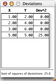
• The sum of squares of deviations is shown at the top of the applet. The closer this number is to zero the more accurate your function is in relation to your data. You may see a data table of these deviations by clicking the Show Deviations button.
  
• Checking the Show Squares check box draws squares from the data points to the function on the coordinate plane. The length of each side of the square is equal to the vertical distance from the coordinate to the function value at the x-value of the coordinate.
  
• Decreasing the sum of the squares of the deviations between the points and the function (think of decreasing the sum of the areas of the squares shown above) produces a better "fit" of the function to the data. Experiment by moving the sliders from side to side until you find a value that you think minimizes the sum of squares of deviations:
  

Description

This activity allows the user to plot data points and functions on the same coordinate plane. This activity would work well in groups of three to four students for about 45 minutes if you use the exploration questions. Time will also vary depending on how many data sets you use.

Place in Mathematics Curriculum

This activity can be used to:

• Develop understanding of the Cartesian coordinate system
• Explore how changing coefficients affects the shape of a graph.

Be Prepared to

• explain how to decide what type of relationship a set of data have
• give examples of real world situations where people try to fit a line to a set of data
• generalize the effects of changing the constants in the type of function the students are studying

Related Resources

• Activity Conic Flyer
• Activity Data Flyer
• Activity Derivate
• Activity Function Flyer
• Activity Function Revolution
• Activity Graphit
• Activity InteGreat!
• Activity Multiple Linear Regression
• Activity Overlapping Gaussians
• Discussion about From Graphs to Function Machines and Back
• Discussion about Functions as Processes or Rules: "Function Machines"
• Discussion about Independent and Dependent Variables
• Lesson on Derivate
• Lesson on Linear Regression and Correlation
• Worksheet Multi-Function Data Flyer Exploration Questions
• Worksheet Multi-Function Data Flyer Exploration Questions (doc)